Searchlights 
In univariate analyses there is a distinction between whole-brain and ROI-based analyses. When done correctly, whole-brain univariate analyses allow you to identify, in an unbiased and data-driven way, regions of the brain that differ between experimental conditions. Compare this to what we have done with multivariate classification: up to this point we have taken ROIs (e.g., FFA, PPA, even the whole brain) and looked at the pattern of activity across voxels. Using these procedures we have been able to determine whether these voxels collectively contain information about different conditions. However, throughout these analyses it has been unclear whether a subset of these voxels have been driving classification accuracy. Although we could use the weights to indicate which voxels are important, weights alone do not always convey the influence of individual voxels. In other words, we have been unable to say with certainty where in the brain there are representations that distinguish between conditions.
A searchlight is a spatial moving window that exhaustively searches the brain in order to localize representations. Running a searchlight is computationally intensive because it involves running a separate multivariate analysis for every voxel in the brain. Imagine doing your feature selection, hyper-parameter optimization, and cross-validation 100,000 times or more. Fortunately, BrainIAK contains a procedure that efficiently carves up brain data into appropriate chunks and distributes them across the computational resources available.
For more information on the searchlight technique, read this comprehensive NeuroImage Comment, that also includes citations to landmark papers on the topic. The validity of using searchlights is explained here.
Pre-requisites: Familiarity with data loading and classification, notebooks 1-5.
Goal of this script
- Learn how to perform a whole-brain searchlight.
- Learn how to replace the kernel used inside the searchlight.
- Use batch scripts, SLURM, and MPI to run searchlight on compute clusters.
- Run searchlight on a face-scene dataset.
Table of contents
Dataset 
For this script we will use the face/scene dataset from Wang et al. (2015), who in turn used localizer data from Turk-Browne et al. (2012).
Localizer details from Turk-Browne et al. (2012):
"Subjects also completed a functional localizer run lasting 6 min 6 s [...] The localizer run alternated between six repetitions each of scene and face blocks (Turk-Browne et al., 2010). Blocks contained 12 stimuli presented for 500 ms every 1500 ms. The 18 s of stimulation was followed by 12 s of fixation before the next block. Subjects made the same indoor/outdoor judgment for scenes, and a male/female judgment for faces."
Self-study: Explore the data
1. Searchlight workflow 
Running a searchlight is computationally intensive, complex and involves many steps. To show how the searchlight functionality in BrainIAK works, we will walk through the steps needed to perform a simple searchlight that can be run in this notebook before moving onto a real example that requires submitting the job to a cluster. This simple workflow takes the following steps:
However, before we start, there are a few things that you should know about searchlights. Think of a searchlight as a processing step in which you pull out a certain size chunk of your data and then perform a kernel operation (specified by a function you write). You can use any kernel on this chunk of data interchangeably. Critically, the searchlight function does not specify the analysis you want to perform, all it does is carve up the data.
Computational demand and parallelization
As mentioned before, searchlights are computationally intensive and so we need to be aware of what kind of burden they might impose. With each subject, we want to perform the operation thousands of times (once for each of their brain voxels). If we were to run this serially, even if each operation only took 1 s to complete, the analysis would take multiple days for only one participant. With nested cross-validation or other recursive steps, the full analysis could take months or years (and you'd lose a lot of points on your assignment).
Fortunately, the searchlight function in BrainIAK intelligently parallelizes your data to give you a considerable and scalable speed boost. Parallelization is the idea that when two or more computational tasks can be completed independently (because they don't interact in any way) then it is possible to run these tasks simultaneously on different cores. Note that we refer to cores as our unit of serial processing, although there are other parallelizations available within-core, such as threads or even multiple instructions within thread. The nice thing about parallelization is that it is scalable: in general, a job parallelized across 10 cores will run up to 10 times faster than on one core. For reference, your computer likely has 2, 4, or more cores, so you could speed up processing if you recruited all of these resources (and shut down all other types of background processing).
How does the BrainIAK searchlight work?
To analyze data efficiently, it is important to understand how the Searchlight function in BrainIAK works. You must provide the function with a numpy volume of 4D data and a binary mask of brain voxels. The searchlight code simply searches for every voxel in the mask that is equal to 1 and then centers a searchlight around this. This means that for every value of 1 in your mask, the searchlight function will apply your kernel function to the corresponding voxel (and those around it) in the 4D volume. Hence when writing the kernel you need to keep in mind that the input data the function receives are not the size of the original data but instead the size of the searchlight radius. In other words, you might give the searchlight function a brain and mask volume that is 64x64x64 but each kernel operation only runs on a data and mask volume that is 3x3x3 (or whatever your searchlight radius is). As per the logic of searchlights, the center of each mask in the searchlight will be equal to 1 (otherwise the searchlight wouldn't have selected it).
How to start using a searchlight? Small!
When getting used to searchlights it is encouraged that you scale up your code gently. This is to prevent the possibility that you run a searchlight that takes a very long time to finish only to find there was a small error (which happens a lot). Instead it is better to write a simple function that runs quickly so you can check if your code works properly before scaling up. A simple workflow for testing your searchlight (and estimating how long your searchlight would take on a bigger dataset) would be this:
- Create a mask of one voxel and run the searchlight interactively (like we are doing now, using a notebook) to check whether the code works.
- Use timestamps to extract the execution time
- Print the number of voxels that are passed to the searchlight function
- Run the searchlight as a job on the smallest unit of real data you have (a single run or single participant)
- Check the runtime and memory usage of this searchlight (e.g. on slurm:
sacct -j $JID --format=jobid,maxvmsize,elapsed).
Taking our own advice, we are going to write a searchlight script below to perform a very simple searchlight. In fact we are only going to run this searchlight on one voxel in the brain so that we can see whether our code is working and how long each kernel operation would take. After we have familiarized ourselves with the way searchlights work on a small scale, we will then graduate to full-scale analyses using batch scripts and cluster computing.
1.1 Data preparation 
Prepare a single participant using a similar pipeline to what we have developed previously. The critical change needed here is the shape of the data: In the past we wanted a time x voxel matrix, but the input to a searchlight is a 4D volume (brain x, y, z, time t), hence we need to add a step, as below.
Exercise 1: Why does the input to a searchlight analysis need to be 4D rather than 2D?
A:
import warnings
import sys
if not sys.warnoptions:
    warnings.simplefilter("ignore")

# Import libraries
import nibabel as nib
import numpy as np
import os
import time
from nilearn import plotting
from brainiak.searchlight.searchlight import Searchlight
from brainiak.fcma.preprocessing import prepare_searchlight_mvpa_data
from brainiak import io
from pathlib import Path
from shutil import copyfile

# Import machine learning libraries
from sklearn.model_selection import StratifiedKFold, GridSearchCV, cross_val_score
from sklearn.svm import SVC

import matplotlib.pyplot as plt
import seaborn as sns

# Set printing precision
np.set_printoptions(precision=2, suppress=True)

# %matplotlib inline
%matplotlib notebook
%autosave 5
sns.set(style = 'white', context='poster', rc={"lines.linewidth": 2.5})
sns.set(palette="colorblind")
1.1.1 Helper functions 
To make it easy for you to achieve the main goals of this notebook, we have created helper functions that perform data extraction from nifti files data, format them into arrays, and prepares the data for the searchlight function.
from utils import fs_data_dir, results_path

print('data dir = %s' % (fs_data_dir))
# Preprocess the raw data and save it to disk.
def preprocess_and_save_data(fs_data_dir, output_path):
    # Set paths
    suffix = 'bet.nii.gz'
    wb_mask_file =  os.path.join(fs_data_dir, 'mask.nii.gz') # whole brain mask
    fs_epoch_file = os.path.join(fs_data_dir, 'fs_epoch_labels.npy')

    # Create an image object that can be efficiently used by the data loader.
    images = io.load_images_from_dir(fs_data_dir, suffix)
    image_files = sorted(Path(fs_data_dir).glob("*" + suffix))

    # Use a path to a mask file to load a binary mask
    wb_mask = io.load_boolean_mask(wb_mask_file)

    # load epoch file
    epoch_list = io.load_labels(fs_epoch_file)

    # Normalize and format the data.
    bold_data_raw, labels = prepare_searchlight_mvpa_data(images, epoch_list)
    labels = np.array(labels)

    # load the whole brain mask
    whole_brain_mask = nib.load(wb_mask_file)
    whole_brain_mask = whole_brain_mask.get_data()
    coords = np.where(whole_brain_mask)  # Where are the non zero values

    # copy the whole brain mask
    copyfile(wb_mask_file, os.path.join(output_path, 'wb_mask.nii.gz'))

    for sub_id in range(18):
        sub = 'sub-%.2d' % (sub_id+1)
        # extract affine
        nii = nib.load(str(image_files[sub_id]))
        affine_mat = nii.affine  # What is the orientation of the data
        dimsize = (3.5, 3.5, 5.0, 1.0)
        # extract data for this subject
        data_i = bold_data_raw[:,:,:,12*sub_id:12*(sub_id+1)]
        label_i = labels[12*sub_id:12*(sub_id+1)]
        # save
        output_dir = os.path.join(output_path, sub)
        if not os.path.exists(output_dir):
            os.makedirs(output_dir)
        output_name = 'data.nii.gz'
        bold_nii = nib.Nifti1Image(data_i, affine_mat)
        hdr = bold_nii.header  # get a handle for the .nii file's header
        hdr.set_zooms((dimsize[0], dimsize[1], dimsize[2], dimsize[3]))
        nib.save(bold_nii, os.path.join(output_dir, output_name))
        np.savez_compressed(os.path.join(output_dir, 'label.npz'),label=label_i)
# Load and perpare data for one subject
def load_fs_data(data_path, sub_id, mask=''):
    # find file path
    sub = 'sub-%.2d' % (sub_id)
    input_dir = os.path.join(data_path, sub)
    data_file = os.path.join(input_dir, 'data.nii.gz')
    label_file =  os.path.join(input_dir, 'label.npz')
    if mask == '':
        mask_file = os.path.join(data_path, 'wb_mask.nii.gz')
    else:
        mask_file = os.path.join(data_path, '{}_mask.nii.gz'.format(mask))

    # load bold data and some header information so that we can save searchlight results later
    data_file = nib.load(data_file)
    bold_data = data_file.get_data()
    affine_mat = data_file.affine
    dimsize = data_file.header.get_zooms()

    # load label
    label = np.load(label_file)
    label = label['label']

    # load mask
    brain_mask = nib.load(mask_file)
    brain_mask = brain_mask.get_data()

    return bold_data, label, brain_mask, affine_mat, dimsize
1.1.2 Create a directory structure 
We strongly recommend storing the data and results generated by the analysis in separate directories from the raw data (here we have enforced this by making the raw data directory read-only). On clusters these kinds of intermediate products should be stored on high-speed scratch disks. Typically, once your analysis is finished, you would copy the results and any important intermediate steps back to more permanent storage like your home directory or a project directory.
Please specify the path to a useable scratch folder:
scratch_folder = results_path
# Set up directories
# Preprocessed data path
data_path = os.path.expanduser(scratch_folder + '/searchlight_data')
if not os.path.exists(data_path):
    os.makedirs(data_path)

# Make directory to save results
output_dir = os.path.expanduser(scratch_folder + '/searchlight_results')
if not os.path.exists(output_dir):
    os.makedirs(output_dir)
1.1.3 Loading, normalizing, and saving the data 
The function preprocess_and_save_data will normalize and save the data to searchlight_data. Some important points to note about this function.
io.load_images_from_dir(data_dir, suffix): This function creates a list of files that need to be loaded. You can load multiple subjects data at once.io.load_boolean_mask: Loads a whole brain mask.prepare_searchlight_mvpa_data: Normalizes and concatenates data from all subjects into a list of arrays. It also concatenates the labels from each subject. Some analysis methods use data across subjects and this step ensures that you are ready for either option.epoch_list: Specifies the timing of blocks from the different experimental conditions [participant,condition,block index,time]. Refer to 09-fcma.ipynb for more detail.
# Before preprocessing the data, let's take a look at the structure of the raw epoch file
fs_epoch_file = os.path.join(fs_data_dir ,'fs_epoch_labels.npy')

# Read in the epoch data from "fs_epoch_labels.npy"
epoch_label = np.load(fs_epoch_file)

# Inspect the shape of the numpy array. Should be (subject, condition, epoch_id, TR)
print(epoch_label.shape)

# Display the first 3 epochs separately as TR sequence in the first participant
# Plot both conditions in the same subplot but with different colors
f, ax = plt.subplots(3,1, figsize = (9, 6))
for ep in range(3):
    ax[ep].plot(epoch_label[0,0,ep,:],'r') # red for condition 0
    ax[ep].plot(epoch_label[0,1,ep,:],'b') # blue for condition 1
    ax[ep].set_title('epoch % s' % ep, fontsize=14)
    ax[ep].tick_params(axis='both', which='major', labelsize=10)
f.tight_layout()

# Call data preprocessing script. You only need to run this line once, even if you have re-run earlier cells.
preprocess_and_save_data(fs_data_dir, data_path)
# Load the data from the first subject
sub_id = 1
bold_vol, labels, whole_brain_mask, affine_mat, dimsize = load_fs_data(data_path, sub_id)
The current face-scene dataset used in this notebook is aligned to standard MNI space. Hence, it is fine to apply the same whole-brain mask to all subjects. Often, we would like to run searchlights in the individual subject space, for example, in previous notebooks we ran decoding on each individual subjects data (that had multiple runs). If that is the case, you can just load subject 4D data in, name it `bold_vol`, along with the subject specific mask named `whole_brain_mask`. We have provided a batch script `./07-searchlight/searchlight_single_subject.py` that implements within subject searchlight analysis.
# Insert code here
1.2 Executing the searchlight workflow
1.2.1 Set searchlight parameters 
To run the searchlight function in BrainIAK you need the following parameters:
- data = The brain data as a 4D volume.
- mask = A binary mask specifying the "center" voxels in the brain around which you want to perform searchlight analyses. A searchlight will be drawn around every voxel with the value of 1. Hence, if you chose to use the wholebrain mask as the mask for the searchlight procedure, the searchlight may include voxels outside of your mask when the "center" voxel is at the border of the mask. It is up to you to decide whether then to include these results.
- bcvar = An additional variable which can be a list, numpy array, dictionary, etc. you want to use in your searchlight kernel. For instance you might want the condition labels so that you can determine to which condition each 3D volume corresponds. If you don't need to broadcast anything, e.g, when doing RSA, set this to 'None'.
- sl_rad = The size of the searchlight's radius, excluding the center voxel. This means the total volume size of the searchlight, if using a cube, is defined as: ((2 * sl_rad) + 1) ^ 3.
- max_blk_edge = When the searchlight function carves the data up into chunks, it doesn't distribute only a single searchlight's worth of data. Instead, it creates a block of data, with the edge length specified by this variable, which determines the number of searchlights to run within a job.
- pool_size = Maximum number of cores running on a block (typically 1).
A:
# Make a mask of only one arbitrary voxel
small_mask = np.zeros(whole_brain_mask.shape)
small_mask[30, 31, 13] = 1

# Preset the variables to be used in the searchlight
data = bold_vol
mask = small_mask
bcvar = labels
sl_rad = 1
max_blk_edge = 5
pool_size = 1

# We will get back to these commands once we finish running a simple searchlight.
#comm = MPI.COMM_WORLD
#rank = comm.rank
#size = comm.size

# Start the clock to time searchlight
begin_time = time.time()
1.2.2 Create Searchlight Object 
# Create the searchlight object
sl = Searchlight(sl_rad=sl_rad,max_blk_edge=max_blk_edge)
print("Setup searchlight inputs")
print("Input data shape: " + str(data.shape))
print("Input mask shape: " + str(mask.shape) + "\n")

# Distribute the information to the searchlights (preparing it to run)
sl.distribute([data], mask)

# Data that is needed for all searchlights is sent to all cores via the sl.broadcast function. In this example, we are sending the labels for classification to all searchlights.
sl.broadcast(bcvar)
1.2.3 Define the function (a.k.a. "kernel") that needs to be computed 
For every searchlight you need a function to run in the searchlight. This is the function that you want to measure/classify your data with. This could perform classification, RSA, or any other computation that you wish.
NB. The word "kernel" is used in multiple mathematical/computational contexts. In this notebook we use kernel to represent the function that is passed to the searchlight object.
# Set up the kernel, in this case an SVM
def calc_svm(data, sl_mask, myrad, bcvar):

    # Pull out the data
    data4D = data[0]
    labels = bcvar

    bolddata_sl = data4D.reshape(sl_mask.shape[0] * sl_mask.shape[1] * sl_mask.shape[2], data[0].shape[3]).T

    # Check if the number of voxels is what you expect.
    print("Searchlight data shape: " + str(data[0].shape))
    print("Searchlight data shape after reshaping: " + str(bolddata_sl.shape))
    print("Searchlight mask shape:" + str(sl_mask.shape) + "\n")
    print("Searchlight mask (note that the center equals 1):\n" + str(sl_mask) + "\n")

    t1 = time.time()
    clf = SVC(kernel='linear', C=1)
    scores = cross_val_score(clf, bolddata_sl, labels, cv=3)
    accuracy = scores.mean()
    t2 = time.time()

    print('Kernel duration: %.2f\n\n' % (t2 - t1))

    return accuracy
1.2.4 Execute the searchlight 
We execute the searchlight and save the results in brain space. Each searchlight result is assigned to the voxel that the searchlight is centered on. This array is then saved to a nifti volume using the following:
nib.Nifti1Image: Created a nifti volume with the same size and in the same space (e.g. MNI) as the subject data.
.header: This gets header information from the subject data.
.set_zooms: Sets the voxel dimensions e.g 1.5mm x 1.5mm x 1.5mm.
print("Begin Searchlight\n")
sl_result = sl.run_searchlight(calc_svm, pool_size=pool_size)
print("End Searchlight\n")

end_time = time.time()

# Print outputs
print("Summarize searchlight results")
print("Number of searchlights run: " + str(len(sl_result[mask==1])))
print("Accuracy for each kernel function: " +str(sl_result[mask==1].astype('double')))
print('Total searchlight duration (including start up time): %.2f' % (end_time - begin_time))

# Save the results to a .nii file
output_name = os.path.join(output_dir, ('subj%s_SL_result.nii.gz' % (sub_id)))
sl_result = sl_result.astype('double')  # Convert the output into a precision format that can be used by other applications
sl_result[np.isnan(sl_result)] = 0  # Exchange nans with zero to ensure compatibility with other applications
sl_nii = nib.Nifti1Image(sl_result, affine_mat)  # create the volume image
hdr = sl_nii.header  # get a handle of the .nii file's header
hdr.set_zooms((dimsize[0], dimsize[1], dimsize[2]))
nib.save(sl_nii, output_name)  # Save the volume
A:
A:
# Insert code here
# Insert code here
Exercise 7: Modify this new calc_svm function to additionally perform nested cross-validation (use the code you made for the notebook on classification) over different cost parameters of the linear SVM kernel. Note that we do not have run_ids as in the previous notebooks, so you should use the StratifiedKFold to perform the cross-validation.
# Insert code here
# Insert code here
# Paste code here for the exercises
Visualizing the data
As you have seen, the output of the searchlight analysis is a 3D volume with the outputs of your kernel for each voxel it was centered on. The nilearn package has multiple plotting options to allow you to view your data within python. This is good for quick visualizations but can be buggy and is not great for exploration. You can also view the data in other packages such as FSL or AFNI. If you followed the steps above, you likely won't see many bright spots because we only ran the searchlight in a tiny part of the brain. But if you look at the data in fslview and change the coordinates to X=30, Y=31, Z=13 you should see a non-zero value.
1.3 Executing on multiple subjects 
So far we have loaded data for one subject and performed within-subject analysis, similar to what we have done in notebooks 1-5 (but in standard MNI space). You can also perform searchlight analysis on a group of subjects. This requires making a list of subjects.
# Load 3 subjects
all_bold = [] # Each subject's data is an element in the list. BrainIAK will handle this format.
all_labels = []
all_affine_mat = []
all_dimsize = []
for sub_id in range(1,4):
    bold_vol, labels, whole_brain_mask, affine_mat, dimsize = load_fs_data(data_path, sub_id)
    all_bold.append(bold_vol)
    all_labels.append(labels)
    all_affine_mat.append(affine_mat)
    all_dimsize.append(dimsize)

# Make a mask of a 4 x 4 x 4 region
small_mask = np.zeros(whole_brain_mask.shape)
small_mask[28:32, 29:33, 11:15] = 1

# Preset the variables
data = all_bold
mask = small_mask
bcvar = all_labels
sl_rad = 1
max_blk_edge = 5
pool_size = 1

# Start the clock to time searchlight
begin_time = time.time()

# Create the searchlight object
sl = Searchlight(sl_rad=sl_rad,max_blk_edge=max_blk_edge)
print("Setup searchlight inputs")
print("Number of subjects: " + str(len(data)))
print("Input data shape: " + str(data[0].shape))
print("Input mask shape: " + str(mask.shape) + "\n")

# Distribute the information to the searchlights (preparing it to run)
sl.distribute(data, mask)
# Data that is needed for all searchlights is sent to all cores via the sl.broadcast function.
#In this example, we are sending the labels for classification to all searchlights.
sl.broadcast(bcvar)
# Set up the kernel, in this case an SVM
def calc_svm(data, sl_mask, myrad, bcvar):
    accuracy = []
    # Loop over subject:
    for idx in range(len(data)):
        # Pull out the data
        data4D = data[idx]
        labels = bcvar[idx]
        bolddata_sl = data4D.reshape(sl_mask.shape[0] * sl_mask.shape[1] * sl_mask.shape[2], data[0].shape[3]).T
        clf = SVC(kernel='linear', C=1)
        scores = cross_val_score(clf, bolddata_sl, labels, cv=3)
        accuracy.append(scores.mean())
    return accuracy

# Execute searchlight on 3 subjects
print("Begin Searchlight\n")
sl_result_3subj = sl.run_searchlight(calc_svm, pool_size=pool_size)
print("End Searchlight\n")
end_time = time.time()
print('Total searchlight duration (including start up time): %.2f' % (end_time - begin_time))
Sanity Check:
To make sure that each subject is being processed correctly, we can compare the results by loading one subject alone vs. loading the same subject amongst three subjects.
# Run it on the first subject alone
data_1 = [all_bold[0]]
bcvar_1 = [all_labels[0]]
begin_time = time.time()

# Create the searchlight object
sl = Searchlight(sl_rad=sl_rad,max_blk_edge=max_blk_edge)

# Distribute the information to the searchlights (preparing it to run)
sl.distribute(data_1, mask)

# Data that is needed for all searchlights is sent to all cores via the sl.broadcast function. In this example, we are sending the labels for classification to all searchlights.
sl.broadcast(bcvar_1)

# Execute searchlight on the first subject
print("Begin Searchlight\n")
sl_result_1subj = sl.run_searchlight(calc_svm, pool_size=pool_size)
print("End Searchlight\n")
end_time = time.time()
print('Total searchlight duration (including start up time): %.2f' % (end_time - begin_time))

# Compare the results using one subject and 3 subjects
# Extract the two accuracy maps
accu_from_1 = np.array([r[0] for r in sl_result_1subj[mask==1]])
accu_from_3 = np.array([r[0] for r in sl_result_3subj[mask==1]])

# Print them out to compare
print("Accuracy for each kernel function from one subject: \n" + str(accu_from_1))
print("\nAccuracy for each kernel function from 3 subjects: \n" + str(accu_from_3))

# compare using numpy
print ('Are the two arrays close: ')
print (np.allclose(accu_from_1, accu_from_3))

# Data format of the accuracy array
print ("\nShape of the accuracy array: " + str(sl_result_3subj.shape))
print ("\nOne element of the accuracy array: "+ str(np.array(sl_result_3subj[30,30,13]))) # each element has the accuracy for 3 subjecs
2. Running searchlight analyses on a cluster
Note: If you are running this section in a non-cluster environment (e.g., a laptop or a server with limited resources), the run-tine for this section can be quite long. You can make an estimate of the run-time (see exercise 4 above) and plan accordingly.
Running searchlight analyses through notebooks or interactive sessions isn't tractable for real studies. Although the example above ran quickly and without parallelization, we only performed 64 analyses. We are now going to write a script to run a searchlight as a "batch" job. To learn how to submit jobs, you need to know a bit about slurm, the scheduling system we assume you are using. If you are using a different scheduler you will need to follw different instructions.
To run a job, a good work flow is to have two scripts: One script that actually does the computation you care about (e.g., a python script like utils.py) and a bash script that sets up the environment and specifies the job parameters. The environment refers to the modules and packages you need to run your job. The job parameters refer to the partition you are going to use (-p), the number of cores (-n), the amount of memory (-m) and required time (-t). To run your job you then call the bash script with something like: 'sbatch script.sh'
Self-study: Lucky for you we have already written the script needed here, called run_searchlight.sh. This script is written in the bash command language. Please explore this script to get familiar with submitting jobs. It will be very useful for future analyses to customize it for your needs (using a text editor like nano or nedit).
# Print the bash script for running searchlights
!cat 07-searchlight/run_searchlight.sh
When a job starts, a log file named as searchlight-%j.out is automatically created in the same directory as your shell script. You can see any output from your script printed into the log file. You can print out the content of the log file in the terminal or open it using a text editor to help debug your code. To check the status of your job you should use squeue -u $USER. Sometimes your jobs won't run immediately because they are waiting in the queue. Conversely, don't submit too many jobs or your classmates won't be able to run theirs.
2.1 Distributing jobs with parallel computing
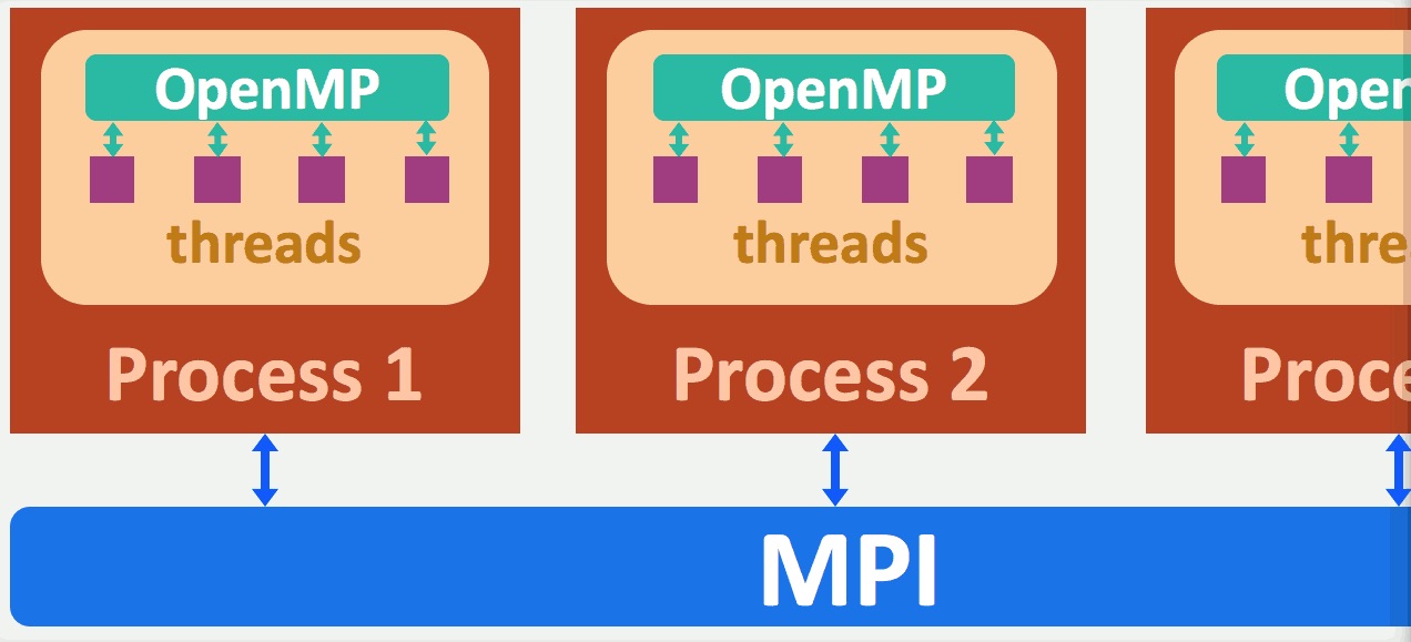
When you parallelize an analysis across multiple cores, this typically means that each core will run the code independently (though there are ways for cores to communicate directly with each other). This means you will load in all of the data on each core. The searchlight function then notices that there are multiple cores running the same job and assigns different pieces of the data to each core for analysis. The message passing interface (MPI), the parallelizing framework used by BrainIAK and most high-performance computing applications, keeps track of each process by assigning it a rank, starting at 0. We provide a brief overview of ranks, cores, and nodes below.
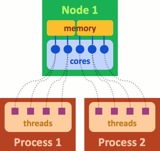
What is a rank? It is a process generated by the application that you are running. In the above figure "Process 1" can be considered to be rank=0 and "Process 2" rank=1. A rank can use more than one core on the cluster and is managed by MPI. Each rank also uses a part of the memory allocated. The cores and memory are part of the hardware belonging to a "node". A node is akin to a server. When you submit a job, you are requesting use of part of the node, or sometimes even the entire node. Optimizing the memory, and number of cores for your batch job will lead to significant gains in run-time for your programs.
MPI handles all communication between the ranks (or processes). This can occur within a single node, or if you have asked for lots of resources, this can even span multiple nodes. Each process can spawn multiple threads, and Open-MP handles communication between threads.
You do not need to configure any of the above. BrainIAK handles all the parallelization for you. Just make sure that you have requested the appropriate number of cores and the memory for your job.
If you are running an analysis across 2 cores then some of your computations will be run with rank=0 and some with rank=1. The following commands are used to access MPI information that your job needs.
comm = MPI.COMM_WORLD
rank = comm.rank
size = comm.size
For efficient utilization of memory, we typically load the data on as few ranks as possible. If memory is sufficient to load all data on one rank, then we would write someting like this:
if rank==0:
    load all my data
else:
    load labels for all subject
    load the mask
distribute(pieces of my data to other ranks)
run searchlight
The above will avoid loading every subjects data on every rank. The labels and mask must be loaded on all ranks. The distribution will allocate only pieces of the data for processing. Again, this is all handled by MPI. In searchlight, the sl.distribute methods handles the distribution to different ranks.
After the searchlights have all finished, you need to save the data. MPI gathers the results from all of the cores and BrainIAK saves the results.
# Example of loading data only one rank.
from mpi4py import MPI
comm = MPI.COMM_WORLD
rank = comm.rank
size = comm.size

sub_id = 1
# Load data only on rank==0
if rank==0:
    bold_vol, labels, whole_brain_mask, affine_mat, dimsize = load_fs_data(data_path, sub_id)
    data = bold_vol
# Make a mask of only one arbitrary voxel
small_mask = np.zeros(whole_brain_mask.shape)
small_mask[28:32, 29:33, 11:15] = 1

# Preset the variables

mask = small_mask
bcvar = labels
sl_rad = 1
max_blk_edge = 5
pool_size = 1


# Start the clock to time searchlight
begin_time = time.time()

# Create the searchlight object
sl = Searchlight(sl_rad=sl_rad,max_blk_edge=max_blk_edge)
print("Setup searchlight inputs")
print("Input data shape: " + str(data.shape))
print("Input mask shape: " + str(mask.shape) + "\n")

# Distribute the information to the searchlights (preparing it to run)
sl.distribute([data], mask)

# Data that is needed for all searchlights is sent to all cores via the sl.broadcast function. In this example, we are sending the labels for classification to all searchlights.
sl.broadcast(bcvar)

# Set up the kernel, in this case an SVM
def calc_svm(data, sl_mask, myrad, bcvar):
    if np.sum(sl_mask) < 14:
        return -1
    # Pull out the data
    data4D = data[0]
    labels = bcvar
    bolddata_sl = data4D.reshape(sl_mask.shape[0] * sl_mask.shape[1] * sl_mask.shape[2], data[0].shape[3]).T
    t1 = time.time()
    scores = []
    # outer loop
    sp = StratifiedKFold(n_splits=3)
    for train, test in sp.split(bolddata_sl, labels):
        train_data = bolddata_sl[train, :]
        test_data = bolddata_sl[test, :]
        train_label = labels[train]
        test_label = labels[test]
        # inner loop
        sp_train = StratifiedKFold(n_splits=2)
        parameters = {'C':[0.01, 0.1, 1, 10]}
        inner_clf = GridSearchCV(
            SVC(kernel='linear'),
            parameters,
            cv=sp_train,
            return_train_score=True)
        inner_clf.fit(train_data, train_label)
        # best C from inner loop
        C_best = inner_clf.best_params_['C']
        # Train in outer loop
        clf = SVC(kernel='linear', C=C_best)
        clf.fit(train_data, train_label)
        # Test in outer loop
        scores.append(clf.score(test_data, test_label))
    accuracy = np.mean(scores)
    t2 = time.time()
#     print('Kernel duration: ' + str(t2 - t1) + "\n\n")
    return accuracy

print("Begin SearchLight\n")
sl_result = sl.run_searchlight(calc_svm, pool_size=pool_size)
print("End SearchLight\n")

end_time = time.time()

# Print outputs
print("Summarize searchlight results")
print("Number of searchlights run: " + str(len(sl_result[mask==1])))
print("Accuracy for each kernel function: " + str(sl_result[mask==1].astype('double')))
print('Total searchlight duration (including start up time): %.2f' % (end_time - begin_time))
We have written a Python script for running searchlights. The file searchlight.py loads in number of participants, sets up the searchlight and kernel and then performs the searchlight across the multiple cores that the code is run on.
This code performs leave-one-subject-out cross validation (i.e., the testing accuracy of subject 1 is based on the SVM classifier trained on subject 2 and 3; accuracy of subject 2 is based on the SVM trained on subject 1 and 3, etc.) The reason we are doing this cross-validation is that the single subject case as in the previous sections in this notebook is a case of double dipping. We only have one run of data for each subject, so the z-scoring within subject will cause double dipping in the single subject case.
These results are saved for each subject separately.
Exercise 10: Run the run_searchlight.sh script using sbatch run_searchlight.sh in the command line. Once your analysis has finished (should take ~6 mins), load in your averaged searchlight results and plot it with the imported function plotting from nilearn. You will find function plotting.plot_stat_map useful. However, be aware that some of these functions assume the brain is MNI space. This face-scene dataset is not in MNI space, so if you overlay it on the default background the image will be 'outside of the brain'. To visualize this correctly, also provide the image as bg_img into this function. Also load in the averaged searchlight results across all 18 subjects we computed for you and plot it. The file is in the same directory as this notebook, called 'avg18_whole_brain_SL.nii.gz'. Use the same 'cut_coords', 'threshold', and 'vmax' across these two plots. You can start from threshold=0.65, cut_coords=(50,-40,10), vmax=1 for a good visualization. Compare the two plots.
Novel contribution: be creative and make one new discovery by adding an analysis, visualization, or optimization.
Some ideas for novel contribution:
- Change the kernel to RSA and correlate it with a model RDM that distinguishes faces and scenes. Compare the RSA results with the decoding results.
- Compute the confusion matrix for each searchlight. You can find useful information about confusion matrix here.
- Run a searchlight, but not on every voxel. Run searchlights only on every third voxel, whole brain.
- Run each subject on a different rank. BrainIAK searchlight has a way to do that.
- Visualize the accuracy map using surface mapping.
Contributions 
M. Kumar, C. Ellis and N. Turk-Browne produced the initial notebook 03/2018
T. Meissner minor edits
H. Zhang preprocessed dataset, add multi-subject section, add multiple exercises, add solutions, other edits
Vineet Bansal provided the MPI diagrams.
David Turner provided extensive input on how to use MPI for efficient running of jobs.
M. Kumar added MPI information and enhanced section contents.
K.A. Norman provided suggestions on the overall content and made edits to this notebook.
C. Ellis implemented updates from cmhn-s19