Hidden Markov Models for Event Segmentation
If asked to give a quick description of a dinner with friends, you might say something like the following: "First, we met outside the restaurant while waiting for our table. Once we got to our table, we continued talking for a bit before we ordered something to drink and a few appetizers. Later, everyone ordered their dinner. The food arrived after some time and we all began eating. Finally, it was time for dessert and we continued chatting with each other until desert arrived. After this, we split the bill and headed out of the restaurant. We said our goodbyes to each other, while waiting for our taxis, and went home." From this description it is clear that the dinner meeting was composed of stages, or events, that occurred sequentially. Furthermore, these events can be perceived at varying scales. At the longest time scale, the entire dinner could be treated as one event. At smaller time scales, subsets of the meeting such as entering the restaurant, taking off coats, being seated, looking at menus and so on, can be treated as different events. At an even smaller scale, the event of entering the restaurant can be broken up into different sub-events. Regardless of scale, all of these accounts share the property that the event can be represented as a sequence of stages.
The goal of this notebook is to explore methods for finding these “sequence-of-stages” representations in the brain. To accomplish this, we use a machine learning technique called Hidden Markov Modeling (HMM). These models assume that your thoughts progress through a sequence of states, one at a time. You can’t directly observe people’s thoughts, so the states are “hidden” (not directly observable). However, you can directly observe BOLD activity. So the full specification of the HMM is that each “hidden” state (corresponding to thinking about a particular stage of an event) has an observable BOLD correlate (specifically, a spatial pattern across voxels). The goal of HMM analysis is to take the BOLD data timeseries and then infer the sequence of states that the participant’s brain went through, based on the BOLD activity. Note that the broadest formulation of an HMM allows all possible transitions between states (e.g., with three states, some probability of transitioning from S1 to S2, S1 to S3, S2 to S1, S2 to S3, S3 to S1, S3 to S2). However, in the formulation of the HMM used here, we will assume that the participant’s brain can only progress forward between adjacent states (S1 to S2, S2 to S3). This more limited formulation of the HMM is well-suited to situations where we know that events proceed in a stereotyped sequence (e.g., we know that the waiter brings the food after you order the food, not the other way around).
In summary: The HMM analysis used here assumes that the time series of BOLD activity was generated by the participant’s brain progressing through a sequence of states, where each state corresponds to a spatial pattern of BOLD activity. Intuitively, when we do HMM analysis, we are trying to identify when the brain has transitioned from one hidden state to another, by looking at the BOLD time series and estimating when the spatial pattern has switched. By fitting HMM with different numbers of hidden states, we can determine how many states a brain region traverses and identify when the transitions occur. Here we will apply the HMM to fMRI data from watching and recalling a movie (from Chen et al., 2017), identifying how different brain regions chunk the movie at different time scales, and examining where in the brain recalling a movie evokes the same sequence of neural patterns as viewing the movie. A full description is given in Baldassano et al. (2017).
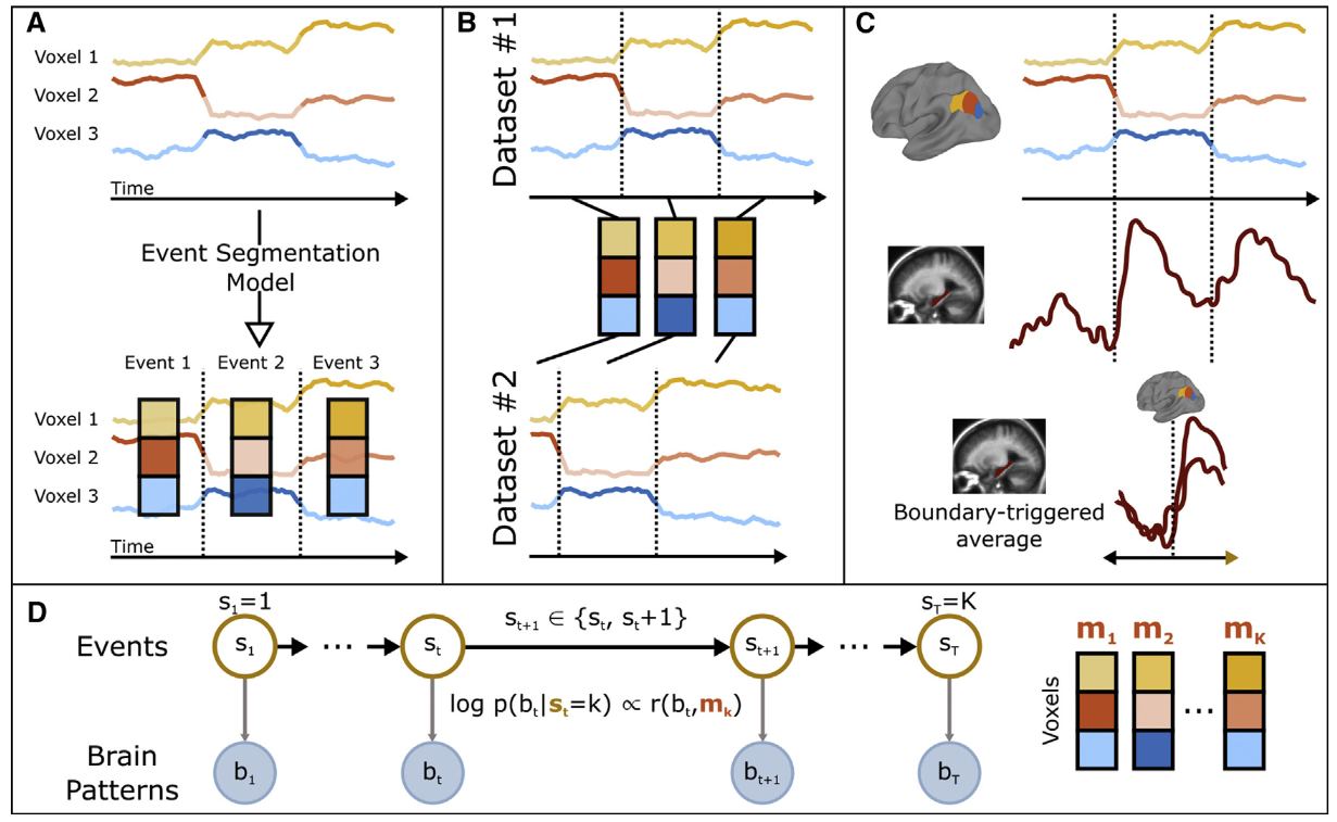
A schematic diagram of HMM, from Baldassano et al. (2017).
- (A) Given a set of (unlabeled) time courses from a region of interest, the goal of the event segmentation model is to temporally divide the data into ‘‘events’’ with stable activity patterns, punctuated by ‘‘event boundaries’’ at which activity patterns rapidly transition to a new stable pattern. The number and locations of these event boundaries can then be compared across brain regions or to stimulus annotations.
- (B) The model can identify event correspondences between datasets (e.g., responses to movie and audio versions of the same narrative) that share the same sequence of event activity patterns, even if the duration of the events is different.
- (C) The model-identified boundaries can also be used to study processing evoked by event transitions, such as changes in hippocampal activity coupled to event transitions in the cortex.
- (D) The event segmentation model is implemented as a modified Hidden Markov Model (HMM) in which the latent state $s_t$ for each time point denotes the event to which that time point belongs, starting in event 1 and ending in event $K$. All datapoints during event $k$ are assumed to be exhibit high similarity with an event-specific pattern $m_k$.
Goal of this script
1. Understand how HMMs can be useful for analyzing time series.
2. Learn how to run HMM in BrainIAK.
3. Use HMM to infer events from brain activity.
4. Determine the statistical significance from the HMM.
Table of Contents
0. HMM with toy data
1. Detect event boundaries from brain activity
1.1. Data loading
1.2. Formal procedure for fitting HMM1.2.1. Inner loop: tune k
1.2.2. Outer loop: statistical testing of boundaries
2. Comparing model boundaries to human-labeled boundaries
3. Aligning movie and recall data
3.1. Fit HMM on the two datasets
3.2. Compare the time scale of events between regions
Exercises
import warnings
import sys
import os
# import logging

import deepdish as dd
import numpy as np

import brainiak.eventseg.event
import nibabel as nib
from nilearn.input_data import NiftiMasker

import scipy.io
from scipy import stats
from scipy.stats import norm, zscore, pearsonr
from scipy.signal import gaussian, convolve
from sklearn import decomposition
from sklearn.model_selection import LeaveOneOut, KFold

from matplotlib import pyplot as plt
from mpl_toolkits.mplot3d import Axes3D
import matplotlib.patches as patches
import seaborn as sns

%autosave 5
%matplotlib inline
sns.set(style = 'white', context='talk', font_scale=1, rc={"lines.linewidth": 2})

if not sys.warnoptions:
    warnings.simplefilter("ignore")

from utils import sherlock_h5_data

if not os.path.exists(sherlock_h5_data):
    os.makedirs(sherlock_h5_data)
    print('Make dir: ', sherlock_h5_data)
else:
    print('Data path exists')

from utils import sherlock_dir
0. HMM with toy data 
Here we introduce the usage of HMM in BrainIAK with a toy simulation. In particular, we will generate data with a known number $K$ of event boundaries. The following steps are used to run this simulation:
- Create event labels for each time-point in the toy dataset using
generate_event_labels.- Create data with these event labels using
generate_data.- Check the data matrix to see if we have created events -- time periods where the signal is relatively constant.
- Segment the signal using the brainiak HMM function:
brainiak.eventseg.event.EventSegment(K).- Overlay the results from HMM with the ground truth segments from the data.
def generate_event_labels(T, K, length_std):
    event_labels = np.zeros(T, dtype=int)
    start_TR = 0
    for e in range(K - 1):
        length = round(
            ((T - start_TR) / (K - e)) * (1 + length_std * np.random.randn()))
        length = min(max(length, 1), T - start_TR - (K - e))
        event_labels[start_TR:(start_TR + length)] = e
        start_TR = start_TR + length
    event_labels[start_TR:] = K - 1

    return event_labels


def generate_data(V, T, event_labels, event_means, noise_std):
    simul_data = np.empty((V, T))
    for t in range(T):
        simul_data[:, t] = stats.multivariate_normal.rvs(
            event_means[:, event_labels[t]], cov=noise_std, size=1)

    simul_data = stats.zscore(simul_data, axis=1, ddof=1)
    return simul_data
Create and plot simulated data. Imagine the following matrix is the voxel by TR bold activity matrix, averaged across participants.
# Parameters for creating small simulated datasets
V = 10 # number of voxels
K = 10 # number of events
T = 500 # Time points

# Generate the first dataset
np.random.seed(1)
event_means = np.random.randn(V, K)
event_labels = generate_event_labels(T, K, 0.2)
D = generate_data(V, T, event_labels, event_means, 1/4)

# Check the data.
f, ax = plt.subplots(1,1, figsize=(12, 4))
ax.imshow(D, interpolation='nearest', cmap='viridis', aspect='auto')
ax.set_ylabel('Voxels')
ax.set_title('Simulated brain activity')
ax.set_xlabel('Timepoints')

The goal of the HMM is to identify chunks of time during which activity patterns remain relatively constant. To see if this is a reasonable model for our dataset, we can plot a timepoint-timepoint correlation matrix, showing the similarity between every pair of timepoints in our dataset (averaged over subjects).
f, ax = plt.subplots(1,1, figsize = (10,8))
ax.imshow(np.corrcoef(D.T), cmap='viridis')
title_text = '''
TR-TR correlation matrix
simulated data
'''
ax.set_title(title_text)
ax.set_xlabel('TR')
ax.set_ylabel('TR')

Calling brainiak.eventseg.event.EventSegment(k) fits a hidden markov model with parameter k, where k is your guess about how many events (or brain states) are in the data. Here we are using the ground truth number of events.
# Find the events in this dataset
hmm_sim = brainiak.eventseg.event.EventSegment(K)
hmm_sim.fit(D.T)
Another output of the event segmentation fit is the estimated activity pattern for each event: HMM.event_pat_.
f, ax = plt.subplots(1,1, figsize=(8, 4))

ax.imshow(hmm_sim.event_pat_.T, cmap='viridis', aspect='auto')
ax.set_title('Estimated brain pattern for each event')
ax.set_ylabel('Event id')
ax.set_xlabel('Voxels')

One way of visualizing the fit is to mark on the timepoint correlation matrix where the model thinks the borders of the events are. The (soft) event segmentation is in HMM.segments_[0], so we can convert this to hard bounds by taking the argmax.
# plot
f, ax = plt.subplots(1,1, figsize=(12,4))

pred_seg = hmm_sim.segments_[0]
ax.imshow(pred_seg.T, aspect='auto', cmap='viridis')
ax.set_xlabel('Timepoints')
ax.set_ylabel('Event label')
ax.set_title('Predicted event segmentation, by HMM with the ground truth n_events')

f.tight_layout()

Exercise 1: What is hmm_sim.segments_[0]? If you sum over event ids, you should get 1 for all TRs. Verify this claim. Why is this the case? Hint: reference BrainIAK documentation.
The field HMM.ll_ stores the log likelihood over optimization steps. A description of what is meant by log-likelihood is provided here.
In the plot below, the likelihood values closer to zero are larger (e.g., -500 > -900) because they are logs. Also note that the HMM is optimized around 120 iterations in this example.
f, ax = plt.subplots(1,1, figsize=(12, 4))

ax.plot(hmm_sim.ll_)
ax.set_title('Log likelihood')
ax.set_xlabel('EM steps')
sns.despine()

Here we overlay the predicted event boundaries on top of the TR-TR similarity matrix, which shows HMM is doing a great job recovering the ground truth.
def plot_tt_similarity_matrix(ax, data_matrix, bounds, n_TRs, title_text):
    ax.imshow(np.corrcoef(data_matrix.T), cmap='viridis')
    ax.set_title(title_text)
    ax.set_xlabel('TR')
    ax.set_ylabel('TR')
    # plot the boundaries
    bounds_aug = np.concatenate(([0],bounds,[n_TRs]))
    for i in range(len(bounds_aug)-1):
        rect = patches.Rectangle(
            (bounds_aug[i],bounds_aug[i]),
            bounds_aug[i+1]-bounds_aug[i],
            bounds_aug[i+1]-bounds_aug[i],
            linewidth=2,edgecolor='w',facecolor='none'
        )
        ax.add_patch(rect)
# extract the boundaries
bounds = np.where(np.diff(np.argmax(pred_seg, axis=1)))[0]

f, ax = plt.subplots(1,1, figsize = (10,8))
title_text = '''
Overlay the predicted event boundaries
on top of the TR-TR correlation matrix
simulated data
'''
plot_tt_similarity_matrix(ax, D, bounds, T, title_text)
f.tight_layout()

1. Detect event boundaries from brain activity 
In this section, we will use HMM on a movie dataset. Subjects were watching the first hour of A Study in Pink, henceforth called the "Sherlock" dataset. Please refer to Chen et al. (2017) to learn more about this dataset.
1.1 Load data 
Download whole-brain data for 17 subjects. Voxels with low inter-subject correlation (that were not consistently activated across subjects) were removed, and then the data were downsampled into 141 large regions (from a resting-state atlas). After putting this .h5 file into the same directory as this notebook, we can load in the data. In addition to the fMRI data, we have the coordinates of each region, as well as human-labeled boundaries for event boundaries.
# download the data, just need to run these lines once
!wget https://ndownloader.figshare.com/files/9017983 -O {sherlock_h5_data}/sherlock.h5
!wget https://ndownloader.figshare.com/files/9055612 -O {sherlock_h5_data}/AG_movie_1recall.h5
D = dd.io.load(os.path.join(sherlock_h5_data, 'sherlock.h5'))
BOLD = D['BOLD']
coords = D['coords']
human_bounds = D['human_bounds']
Exercise 3: Inspect the data. What is BOLD? Which dimension corresponds to number of subjects (nSubj), number of brain regions (nR), and number of TRs (nTR)? Visualize the data for the 1st subject. What is coords? Visualize it with a 3D plot. What is human_bounds? Print out this variable and explain the i-th entry.
# When you complete this exercise, these variables must be filled in.
#nR, nTR, nSubj = ?

1.2 Formal procedure for fitting HMM 
Here, we introduce some rigorous procedures and relevant statistical tests.
We need to pick k - the assumed number of events when fitting HMM. Then, once we figure out what k to use, we need some unseen data to evaluate whether this was a good choice. Therefore we will need to do nested cross-validation. Here is some pseudo code summarizing the procedure:
Given subject 1, subject 2, ... subject N.
Outer loop: Hold out subject i, for i = 1, 2, ..., N, as the final test subject.
Inner loop: For subject j, for all j $\neq$ i, hold out some subjects as the validation set for parameter tuning and use the rest of the subjects as the training set.
For all choices of k, fit HMM on the training set, and compute the log likelihood on the validation set.
Pick the best k (based on the validation set), re-fit the model using subject j, for all j $\neq$ i. And evaluate the the performance of HMM on subject i, the final test subject.
The code block below has the nested cv loop (without fitting HMM) to make things more concrete.
# set up the nested cross validation template
n_splits_inner = 4
subj_id_all = np.array([i for i in range(nSubj)])

# set up outer loop loo structure
loo_outer = LeaveOneOut()
loo_outer.get_n_splits(subj_id_all)
for subj_id_train_outer, subj_id_test_outer in loo_outer.split(subj_id_all):
    print("Outer:\tTrain:", subj_id_train_outer, "Test:", subj_id_test_outer)

    # set up inner loop loo structure
    subj_id_all_inner = subj_id_all[subj_id_train_outer]
    kf = KFold(n_splits=n_splits_inner)
    kf.get_n_splits(subj_id_train_outer)

    print('Inner:')
    for subj_id_train_inner, subj_id_test_inner in kf.split(subj_id_all_inner):
        # inplace update the ids w.r.t. to the inner training set
        subj_id_train_inner = subj_id_all_inner[subj_id_train_inner]
        subj_id_test_inner = subj_id_all_inner[subj_id_test_inner]
        print("-Train:", subj_id_train_inner, "Test:", subj_id_test_inner, ', now try different k...')
    print()
Since the full nested cv procedure is time consuming, we won't do that in this notebook. Instead:
Inner loop - Split the data in a particular way (train / validation / test), fit HMM with different k and evaluate the log likelihood on some unseen subjects.
Outer loop - For a fixed k, fit HMM(k) on some training set, and evaluate HMM(k) on the held-out subject.
1.2.1 Inner loop : tune k 
For some training set and test set, we can train HMM(k) on the training set and evaluate the log likelihood of the trained HMM(k) using the test set. For every k, we will get the a log likelihood.
Then we can pick the k, call it best_k, with the largest log likelihood. If we want to evaluate how good this best_k is, we need other unseen data.
Here, we pick a particular train-test split and try various k.
Exercise 5: Estimate a reasonable value for k, the number of events. Choose a train - validation - test split. Fit HMM with k = 10, 20, ..., 100. Figure out which k works the best based on the log likelihood on the held-out subject by plotting log likelihood against all choices of k. Use the best k to predict event boundaries. Overlay the boundaries on the timepoint-timepoint correlation matrix.
# hold out a subject
subj_id_test = 0
subj_id_val = 1
subj_id_train = [
    subj_id for subj_id in range(nSubj)
    if subj_id not in [subj_id_test, subj_id_val]
]

BOLD_train = BOLD[:,:,subj_id_train]
BOLD_val = BOLD[:,:,subj_id_val]
BOLD_test = BOLD[:,:,subj_id_test]

print('Whole dataset:\t', np.shape(BOLD))
print('Training set:\t', np.shape(BOLD_train))
print('Tune set:\t', np.shape(BOLD_val))
print('Test set:\t', np.shape(BOLD_test))

print(subj_id_train)
print(subj_id_val)
print(subj_id_test)
1.2.2 Outer loop: statistical testing of boundaries 
One way to test whether the model-identified boundaries are consistent across subjects is to fit the model on all but one subject and try to predict something about the held-out subject. There are multiple approaches for doing this (see here), but the simplest is to check whether the model boundaries predict pattern changes in the held-out subject. We therefore measure whether activity patterns 5 TRs apart show a drop in correlation when they are on opposite sides of an event boundary. Here, we pick a k and do the full leave-one-subject-out procedure to test the quality of this choice.
For comparison, we generate permuted versions of the model boundaries, in which the distribution of event lengths (the distances between the boundaries) is held constant but the order of the event lengths is shuffled. This should produce a within vs. across boundary difference of zero on average, but the variance of these null boundaries lets us know the interval of chance values and we can see that we are well above chance.
k = 60
w = 5  # window size
nPerm = 1000

within_across = np.zeros((nSubj, nPerm+1))
for left_out in range(nSubj):
    # Fit to all but one subject
    ev = brainiak.eventseg.event.EventSegment(k)
    ev.fit(BOLD[:,:,np.arange(nSubj) != left_out].mean(2).T)
    events = np.argmax(ev.segments_[0], axis=1)

    # Compute correlations separated by w in time
    corrs = np.zeros(nTR-w)
    for t in range(nTR-w):
        corrs[t] = pearsonr(BOLD[:,t,left_out],BOLD[:,t+w,left_out])[0]
    _, event_lengths = np.unique(events, return_counts=True)

    # Compute within vs across boundary correlations, for real and permuted bounds
    np.random.seed(0)
    for p in range(nPerm+1):
        within = corrs[events[:-w] == events[w:]].mean()
        across = corrs[events[:-w] != events[w:]].mean()
        within_across[left_out, p] = within - across
        #
        perm_lengths = np.random.permutation(event_lengths)
        events = np.zeros(nTR, dtype=np.int)
        events[np.cumsum(perm_lengths[:-1])] = 1
        events = np.cumsum(events)
    print('Subj ' + str(left_out+1) + ': within vs across = ' + str(within_across[left_out,0]))
plt.figure(figsize=(2,5))

plt.violinplot(within_across[:,1:].mean(0), showextrema=False)
plt.scatter(1, within_across[:,0].mean(0))
plt.gca().xaxis.set_visible(False)

plt.ylabel('Within vs across boundary correlation')

2. Comparing model boundaries to human-labeled boundaries 
We can also compare the event boundaries from the model to human-labeled event boundaries. Because there is some ambiguity in both the stimulus and the model about exactly which timepoint the transition occurs at, we will count two boundaries as being a "match" if they are within 3 TRs (4.5 seconds) of each other.
To determine whether the match is statistically significant, we generate permuted versions of the model boundaries as in Section 1.2.2. This gives as a null model for comparison: how often will a human and model bound be within 3 TRs of each other by chance?
np.random.seed(0)

event_counts = np.diff(np.concatenate(([0],bounds,[nTR])))
nPerm = 1000
perm_bounds = bounds
threshold = 3

match = np.zeros(nPerm+1)
for p in range(nPerm+1):
    for hb in human_bounds:
        # check if match
        if np.any(np.abs(perm_bounds - hb) <= threshold):
            match[p] += 1
    match[p] /= len(human_bounds)
    perm_counts = np.random.permutation(event_counts)
    perm_bounds = np.cumsum(perm_counts)[:-1]

plt.figure(figsize=(2,4))
plt.violinplot(match[1:], showextrema=False)
plt.scatter(1, match[0])
plt.gca().xaxis.set_visible(False)
plt.ylabel('Human-model match')
print('p = ' + str(norm.sf((match[0]-match[1:].mean())/match[1:].std())))

3. Aligning movie and recall data 
A simple model of free recall is that a subject will revisit the same sequence of events experienced during perception, but the lengths of the events will not be identical between perception and recall. We can fit this model by separately estimating event boundaries in movie and recall data, while constraining the event patterns to be the same across the two datasets.
We will now download data consisting of (group-averaged) movie-watching data and free recall data for a single subject. These data are from the angular gyrus. We also have a human-labeled correspondence between the movie and recall (based on the transcript of the subject's verbal recall). The full dataset for all 17 subjects is available here.
D = dd.io.load(os.path.join(sherlock_h5_data,'AG_movie_1recall.h5'))

movie = D['movie']
recall = D['recall']
movie_labels = D['movie_labels']
recall_labels = D['recall_labels']
3.1. Fit HMM on the two datasets 
We use the same fit function as for a single dataset, but now we pass in both the movie and recall datasets in a list. We assume the two datasets have shared event transitions.
# fit event seg models
k = 25
hmm_ag_mvr = brainiak.eventseg.event.EventSegment(k)
hmm_ag_mvr.fit([movie.T, recall.T])
This divides the movie and recall into 25 corresponding events, with the same 25 event patterns. We can plot the probability that each timepoint is in a particular event.
plt.figure(figsize=(16, 5))
plt.subplot(1,2,1)
plt.imshow(hmm_ag_mvr.segments_[0].T,aspect='auto',origin='lower',cmap='viridis')
plt.xlabel('Movie TRs')
plt.ylabel('Events')

plt.subplot(1,2,2)
plt.imshow(hmm_ag_mvr.segments_[1].T,aspect='auto',origin='lower',cmap='viridis')
plt.xlabel('Recall TRs')
plt.ylabel('Events')

To get the temporal correspondence between the movie and the recall, we need to find the probability that a movie TR and a recall TR are in the same event (regardless of which event it is):
$$ \sum_k p(T_M == k) \cdot p(T_R == k) $$which we can compute by a simple matrix multiplication.
For comparison, we also plot the human-labeled correspondence as white boxes.
f, ax = plt.subplots(1,1, figsize=(10,8))

ax.imshow(
    np.dot(hmm_ag_mvr.segments_[1], hmm_ag_mvr.segments_[0].T),
    origin='lower',cmap='viridis'
)

# overlay the boundaries
for i in np.unique(movie_labels[movie_labels>0]):
    if not np.any(recall_labels==i):
        continue
    movie_start = np.where(movie_labels==i)[0][0]
    movie_end = np.where(movie_labels==i)[0][-1]
    recall_start = np.where(recall_labels==i)[0][0]
    recall_end = np.where(recall_labels==i)[0][-1]

    rect = patches.Rectangle(
        (movie_start-0.5, recall_start-0.5),
        movie_end - movie_start + 1,
        recall_end - recall_start + 1,
        linewidth=1,edgecolor='w',facecolor='none'
    )
    ax.add_patch(rect)
ax.set_xlabel('Movie TRs')
ax.set_ylabel('Recall TRs')

title_text = """
Estimated temporal correspondence, movie vs. recall
human labels overlayed as bounding boxes
ROI = AG
"""
ax.set_title(title_text)

3.2 Compare the time scale of events between regions. 
Run HMM on two ROIs that correspond to semantic cognition (posterior medial cortex) and sensory processing (auditory cortex). These regions show differences in their time scale of representation.
def load_labels(subj_id):
    label_fname = 'labels_subj%d.mat' % subj_id
    labels = scipy.io.loadmat(os.path.join(sherlock_dir, 'labels', label_fname))
    recall_times = labels['recall_scenetimes']
    movie_times = labels['subj_movie_scenetimes']
    return recall_times, movie_times

def read_sherlock_mat_data(fpath):
    temp = scipy.io.loadmat(fpath)
    return temp['rdata'].T
subj_id = 2

data_dir_subj = os.path.join(sherlock_dir, 'data_mat', 's%d'%subj_id)
recall_dir = os.path.join(data_dir_subj, 'sherlock_recall')
movie_dir = os.path.join(data_dir_subj, 'sherlock_movie')

# load data
fpath_aud_movie  = os.path.join(movie_dir, 'aud_early_sherlock_movie_s%d.mat'%subj_id)
fpath_aud_recall = os.path.join(recall_dir, 'aud_early_sherlock_recall_s%d.mat'%subj_id)

fpath_pmc_movie  = os.path.join(movie_dir, 'pmc_nn_sherlock_movie_s%d.mat'%subj_id)
fpath_pmc_recall = os.path.join(recall_dir, 'pmc_nn_sherlock_recall_s%d.mat'%subj_id)

data_aud_movie = read_sherlock_mat_data(fpath_aud_movie)
data_aud_recall = read_sherlock_mat_data(fpath_aud_recall)

data_pmc_movie = read_sherlock_mat_data(fpath_pmc_movie)
data_pmc_recall = read_sherlock_mat_data(fpath_pmc_recall)

# load labels
recall_times, movie_times = load_labels(subj_id)
Recommended readings
Anderson, J. R., Pyke, A. A., & Fincham, J. M. (2016). Hidden stages of cognition revealed in patterns of brain activation. Psychological Science, 27(9), 1215–1226. https://doi.org/10.1177/0956797616654912
Baldassano, C., Hasson, U., & Norman, K. A. (2018). Representation of real-world event schemas during narrative perception. The Journal of Neuroscience: The Official Journal of the Society for Neuroscience, 38(45), 9689–9699. https://doi.org/10.1523/JNEUROSCI.0251-18.2018
Manning, J. R., Fitzpatrick, P. C., & Heusser, A. C. (2018). How is experience transformed into memory? bioRxiv. https://doi.org/10.1101/409987
Contributions 
- Chris Baldassano developed the initial notebook for brainiak demo.
- Q add exs; nested cv; tune k; modularize code.
- M. Kumar added introduction and edited section descriptions.
- K.A. Norman provided suggestions on the overall content and made edits to this notebook.